Visual SLAM – Bundle Adjustment

1. Foundation
In feature point-based visual SLAM, we generally optimize the camera pose and map point location by minimizing the reprojection error. The following is an introduction to this issue.
1.1 Map parameterise
Two method: 3-d vector $X=\left[ x,y,z \right]^{T}$ , or inverse depth parametrization. Here we use 3-d vector for simplicity.
1.2 Camera model
Use pin-hole model:
$$
\lambda{u}=KTX= \begin{bmatrix}
f_{x} & 0 & c_{x} \\\
0 & f_{y} & c_{y} \\\
0 & 0 & 1
\end{bmatrix} \left[ \begin{array}{cc} R & t \end{array} \right]\begin{bmatrix}
x\\\
y \\\
z \\\
1
\end{bmatrix} \tag{1}
$$

T is camera pose, K is intrinsic. Assume K is known, then this can be simplified to
$$u=\pi{(T,X)}\tag{2}$$

1.3 Residue: a least square problem
$$
\left\{ T_{i},X_{j} \right\}
= arg min \sum_{\left\{i,j,k\right\}\in\chi}{\rho\left({\begin{Vmatrix} \underbrace{z_{k}-\pi\left({T_{i},X_{j}}\right)}_e\end{Vmatrix}}^2_{\sum} \right)} \\
= arg min \sum_{ \left\{i,j,k\right\}\in\chi} {\rho\left( e^{T}{\sum}^{-1}e \right) } \tag{3}
$$

camera pose $T_{i}$ and map point $X_{j}$ are to be optimised, $\chi$ includes all 3D to 2D projection. $e$ is cost function. $\rho$ is robust kernel, here we use Huber function:
$$
\rho = \begin{cases} x &,if\sqrt{x}<{b} \\ 2b\sqrt{x}-b^2 &,else \end{cases}\tag{4}
$$

for convenience, we change $\rho$ to a weight $w$ --   same as g2o does, hence:
$$
e^{T}(w{\sum}^{-1})e = \rho(e^{T}{\sum}^{-1}e)\tag{5}
$$

Then weight $w$ is
$$
w=\frac{\rho({e^{T}{\sum}^{-1}e})}{e^{T}{\sum}^{-1}e}\tag{6}
$$
now the least squares problem become:
$$
\left\{ T_{i},X_{j} \right\} = argmin \sum_{ \left\{i,j,k\right\}\in\chi} { e^{T}(w{\Sigma}^{-1})e } \tag{7}
$$

1.4 Jacobian
To solve the least square problem, we need Jacobian of cost function $e=z-\pi(T,X)$ respect to T and X.
cost function's Jacobian about T, using perturbation theory:
$$
J_T=\begin{bmatrix} \frac{f_x}{z^{'}} &0 &-\frac{{f_x}x^{'}}{{z^{'}}^2} &-\frac{{f_x}x^{'}y^{'}}{{z^{'}}^2} &f_x+\frac{{f_x}{x^{'}}^2}{{z^{'}}^2} &-\frac{{f_x}y^{'}}{z^{'}}\\\ 0 &\frac{f_y}{z^{'}} &-\frac{{f_y}y^{'}}{{z^{'}}^2} &-f_y-\frac{{f_y}{y^{'}}^2}{{z^{'}}^2} &-\frac{{f_y}x^{'}y^{'}}{{z^{'}}^2} &\frac{{f_y}x^{'}}{z^{'}} \end{bmatrix} \tag{8}
$$
where
$$
\begin{bmatrix} x^{'}\\\ y^{'}\\\ z^{'} \end{bmatrix} = \begin{bmatrix}R &t\end{bmatrix} \begin{bmatrix} x\\\ y\\\ z\\\ 1 \end{bmatrix} \tag{9}
$$
2. cost function's Jacobian about map point X :
$$
J_x=-\begin{bmatrix} \frac{f_x}{z^{'}} &0 &-\frac{{f_x}x^{'}}{{z^{'}}^2}\\\ 0 &\frac{f_y}{z^{'}} &-\frac{{f_y}y^{'}}{{z^{'}}^2} \end{bmatrix} \tag{10}
$$

1.5 solve least squares problem
No matter Gauss-Newton or Levenberg–Marquardt algorithm(LM) , we need to solve this linear function:
$$ H{\Delta}X = b\tag{11} $$
where $H\equiv{J_x^{T}J_x}$ and $b\equiv{-J_x}^Tf(x)$.   $H$ is sparse as picture shows.

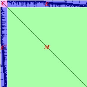
H matrix

As picture shows sub-block C is only related to camera, and block M are related to map point. Both C and M are diagnose matrix. Reformat $(11)$:
$$
\begin{bmatrix} C&E\\\ E^T&M \end{bmatrix} \begin{bmatrix} \Delta{x_c}\\\ \Delta{x_m} \end{bmatrix} =\begin{bmatrix} b_c\\\ b_m \end{bmatrix} \tag{12}
$$
To get $\Delta x_c$ using Shur Compliment:
$$
\begin{bmatrix} C&-EM^{-1}E^T \end{bmatrix} \Delta x_c = b_c - EM^{-1} b_m\tag{12-a}
$$
Then get $\Delta x_p$ :
$$
\Delta x_m=M^{-1}(b_m-E^{T}\Delta x_c)\tag{12-b}
$$
M is diagonal, so its invert operation is fast.

1.6 Fixed state
For a Bundle Adjustment problem, we have to fix a part of the state, or give a prior to a part of the state. Otherwise, there will be infinite solutions. It can be imagined that after the error of a network has reached the minimum, it can move arbitrarily in the space as a whole without causing any effect on the error. As long as we fix any one or more nodes in this network, other nodes will have a definite state. Usually we fix the first pose.
One way to add a prior constraint is to add a prior cost function. The other is to fix the state directly and not let it participate in the optimisation. We take the latter approach.

1.7 Implementation
This implementation is relatively simple, a lot of improvement can be done:

• scalability
• memory usage. Ignored that the matrix is sparse, it occupies a lot of memory, and can only be used to solve small-scale problems.
• acceleration of sparse matrix
• Only implements the LM optimization algorithm so far
• Does not support a priori constraints, there are three forms of motion only BA, struct only BA and Full BA.
• flexible input.
• Speed. This implement refers to the practice of g2o.

2 Test
In order to be able to compare with the real value, I used a simulation experiment. It is to artificially simulate m cameras, n map points and some observations. Then add some noise to the data to test the effectiveness of the algorithm. The simulation experiment has clear ground truth, and the debugger is very easy to use. The results for a set of data are given below.

Number of cameras: 6
Number of map points: 275
Number of observations: 1650

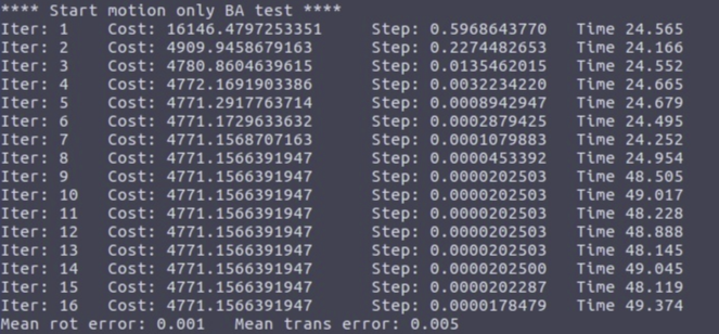
2.1 motion only BA test（fixed map points，optimize pose only）
First, we can experiment without adding any noise, and we can find that the optimized result is exactly the same as the true value. Then, add noise as shown below to test

mpt_noise = 0.01; // dist
cam_trans_noise = 0.1; // dist
cam_rot_noise = 0.1; // rad
ob_noise = 1.0; // pixel

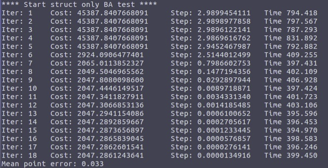
2.2 struct only BA (fixed camera pose, optimize map point)
Add noise:

mpt_noise = 0.1;
cam_trans_noise = 0.0;//camera fixed
cam_rot_noise = 0.00;
ob_noise = 1.0;

3.3 Full BA test（fixed the first camera，optimize other cameras and map points）
test with noise added:

mpt_noise = 0.05;
cam_trans_noise = 0.1;
cam_rot_noise = 0.1;
ob_noise = 1.0;

It is found that the algorithm can converge well. The estimation accuracy of camera pose will be higher than that of map points, because a camera can see hundreds of map points, and a map point can only be seen by a few cameras; the number of camera constraints is much larger than that of map points. Constrain the number of equations. It is also found that the calculation speed is very slow, the main reasons are:

1. memory copy
2. The incremental equation solving speed is slow
3. The properties of the sparse matrix are ignored
4. The way of using Eigen library...